Climate change scenarios over Southeast Asia
Keywords
Climate change · Global climate model (GCM) · Precipitation · Southeast Asia · Surface temperature · Weather research forecast (WRF)
Highlights
- Southeast Asia is at risk from climate change in the next 20 years due to the region’s long coastlines, growing economic activities and population, abundant low-lying areas, and reliance on the agricultural sector, making the area under threat of climate change.
- Climate model simulations indicate that average annual temperatures are likely to increase across the Southeast Asia region by approximately 1°C through 2030 and will keep increasing throughout the century.
- The trends of future precipitation changes showed decrement patterns and varied geographically and temporally across the region in the next 20 years.
1. Introduction
Surface temperature in climate research has shown the most observable indications of variations arising from climate change. This is due to the availability of long observational records, a significant response to anthropogenic forcing, and a strong theoretical understanding of the key thermodynamic driving of its changes (IPCC, 2021). As strongly suggested in the synthesis report of Article 5 of (IPCC, 2018), it is highly likely that the observed increase in global mean surface temperature from early 1950 to 2010 has been caused by human activities (Flato et al., 2013; IPCC, 2021; Shepherd, 2014). Despite that, the rate of warming reduced from 1998 to 2012 due to strong aerosol cooling (Palmer & Stevens, 2019) and an overestimated warming rate (Flynn & Mauritsen, 2020; Golaz et al., 2019). In the Asian region, there is compelling evidence that there has been an increase in the intensity and frequency of extreme heat events and a decrease in the intensity and frequency of extreme cold events in recent decades (Alexander, 2016; Dunn et al., 2020; Imada, Watanabe, Kawase, Shiogama, & Arai, 2019). There is less to be argued for this as, according to (Chen & Zhai, 2017), (Yin, Ma, & Wu, 2018), and (Qian, Zhang, & Li, 2019), using regional studies in East Asia found that there was a warming trend in daily temperatures and an increase in extreme heat frequency since the beginning of the 20th century over the region. In west Asia, there is high confidence found in the studies of (Erlat & Türkeş, 2016), (Imada et al., 2017), (Rahimi-Moghaddam, Kambouzia, & Deihimfard, 2018), and (Rahimi & Hejabi, 2018), suggesting that the frequency of cold events decreased but the warm season lengthened in most of the region.
The climate conditions in the SEA region can be categorized into two seasons: the winter season during the northeast monsoon and the summer season during the southeast monsoon (Rahman et al., 2015). The averages temperatures in Malaysia, the Philippines, and Thailand from 1971 to 2000 were in the range of 27.0°C to 27.8°C (Torsri, Octaviani, Manomaiphiboon, & Towprayoon, 2013), while the average temperatures in Cambodia, Vietnam, and Laos were in the range of 24°C to 28.4°C (World Bank, 2011). According to (IPCC, 2018) , the average surface temperature has increased by between 0.1°C and 0.3°C per decade across the SEA region. In April 2016, the SEA region’s surface temperature, particularly for Cambodia, Laos, Myanmar, Thailand, Vietnam, and Peninsular Malaysia, surpassed the national record with an increment of over 2.0°C, caused by the strong El-Niño (Thirumalai, Dinezio, Okumura, & Deser, 2017). Global climate change has already had observable effects on Earth: sea ice loss, sea-level rise, intense heat waves, and coastal inundation. Although the global temperature will keep rising in the upcoming decade due to human activities, as suggested, the future evolution of the Earth’s climate and its response to the present rapid rate of the increasing trend of CO2 has no precise analogues in the past. It cannot be well understood through laboratory experiments (Hollis et al., 2019). To simulate the patterns, trends, and variability of surface temperature and the impact of human influence on changes in surface temperature, climate models have been used to reproduce large-scale climate variability over a time scale (McClymont et al., 2020).
Climate models are based on mathematical equations that represent the understanding of the fundamental laws of physics, chemistry, and biology that govern the behaviour of the atmosphere, oceans, land surface, ice, and other parts of the climate system. According to (IPCC, 2021), climate models need to represent the response of physical principles and the response of surface temperatures both to external forcing to be fit for detecting and simulating the impact of anthropogenic activities on global or regional surface temperatures over various time scales. A better understanding of climate uncertainties and the forcing applied to model simulation can lead to better simulation of surface temperatures and reconstruction of past climates (Haywood et al., 2020; Lunt et al., 2021) . Several different types of climate models can be used for climate change studies. Each model has different characteristics and functions that run on different climate scenarios and simulate projections of various parameters. The Global Climate Model (GCM) is primarily used to study weather and climate systems. With the climate forcing scenario, GCM can be used to investigate future climate behaviour (Lembo, Lucarini, & Ragone, 2020).
Furthermore, the construction of GCM is based on the physical properties of its components, interactions, and feedback processes that provide climate projections with a scale of a few hundred kilometres. Therefore, the output of this GCM is often in coarse resolution and inefficient at resolving complex terrains, islands, and coastlines (Jones, Forbes, Hagan, & Maute, 2014). Therefore, downscaling to a regional scale for higher resolution by a statistical and dynamic downscaling method using the Regional Climate Modelling (RCM) system was used for a more refined resolution model to overcome the limitations of GCM (Jeong, St-Hilaire, Ouarda, & Gachon, 2012; Sachindra, Huang, Barton, & Perera, 2014) . In addition, the primary purpose of this study is to establish the link between the climate change trends and the dynamics of Asian monsoon seasons and how it impacts the temperature and rainfall variability in the Southeast Asian region.
2. Methodology
2.1 Experimental design
The simulations were carried out in one nested horizontal domain in this study. The domain covered the Southeast Asia region, with 1-hour temporal resolution and 30 km x 30 km spatial resolution. The year 2013 was a neutral year for the El Niño–Southern Oscillation (ENSO) and was selected as the base year of the present-day simulation, and the future projection was for the years 2030, 2050, 2070, and 2100. The simulation was carried out for January and July of the selected years. For January, the projection started at 0000 UTC on the first of January and ended at 0000 UTC on the first of February. While for July, the projection time began at 0000 UTC on the first of July and ended at 0000 UTC on the first of August.
2.2 Dataset input: Initial boundary conditions
This study applied two time-dependent meteorological fields as initial and boundary conditions for the WRF model. For the present-day simulation, the time-dependent meteorological field was obtained from the global NCEP FNL (https://rda.ucar.edu/datasets/ds083.2), as mentioned. The NCEP FNL dataset consists of surface information with 26 mandatory levels (1000 millibars–10 millibars) of the surface boundary level. The meteorological parameters include the surface temperature, sea surface temperature, sea-level pressure, geopotential height, relative humidity, ice cover, vertical motion, vorticity, and winds (National Centers for Environmental Prediction, 1994). While for the future simulations, the NCAR’s Community Earth System Model (CESM) from global bias-corrected climate model output datasets (Hurrell et al., 2013) was used and was obtained from (https://rda.ucar.edu/datasets/ds316.1). These future initial and boundary condition information were then downscaled into 30 km x 30 km resolution to fit for regional projection using the WRF model. In support of Coupled Model Intercomparison Experiment Phase 5 (CMIP5) (Taylor, Stouffer, & Meehl, 2012) and the Intergovernmental Panel on Climate Change Fifth Assessment Report (Flato et al., 2013), the CESM simulations, therefore, were utilized to produce future-day simulation, which has a better agreement in simulating temperature and precipitation globally compared with real-time observations (Knutti, Masson, & Gettelman, 2013).
2.3 Climate change scenarios
This study utilizes the climate change scenario that the IPCC developed in their Fifth Assessment Report (Flato et al., 2013). The climate change scenario provides more comprehensive external forcing scenarios and higher resolution than CMIP3 from IPCC AR4 (Knutti & Sedlacek, 2013). In this study, only two climate scenarios were used and discussed, namely the RCP4.5 and RCP8.5. The RCPs are input for climate and atmospheric chemistry modelling that documents the emissions, concentrations, and land-cover change projections. The four RCPs (RCP2.6, 4.5, 6.0, and 8.5) reflect the year 2100 greenhouse gas radiative forcing values from 2.6 to 8.5 Wm-2 (Nazarenko et al., 2015). The RCPs include the lowest forcing level scenario RCP2.6 (Vuuren et al., 2011), two median range or stabilization scenarios RCP4.5 (Thomson et al., 2011) and RCP6.0 (Masui et al., 2011), and the high-end or business-as-usual scenario RCP8.5 (Riahi et al., 2011). The future scenario of RCP4.5 applied in this study is a low-to-moderate emission scenario, where the greenhouse gases (GHGs) radiative forcing will reach 4.5 Wm-2 by the year 2100 (Thomson et al., 2011). It represents a scenario where various adaptive policies have been applied to limit the radiative forcing. At the same time, RCP8.5 indicates a higher emission scenario with GHGs radiative forcing that will reach 8.5 Wm-2 by the year 2100 (Riahi et al., 2011).
2.4 Climate model evaluation
Most researchers apply dynamical downscaling by RCMs from GCMs due to the uncertainties embedded within the GCMs, especially when resolving complex terrain (IPCC, 2001). Moreover, the error of GCMs with large-scale resolution can be transmitted to the RCM (Noguer, Jones, & Murphy, 1998). As a result, the validation or evaluation process is necessary for RCM, downscaled from GCMs before using it for the climate projection. The evaluation was carried out with observation datasets from the Climate Research Unit (CRU), University of East Anglia. The dataset spaced at 0.5° × 0.5° resolution contained with full-set monthly mean surface climate (Harris, Jones, Osborn, & Lister, 2010). Since the spatial resolution and grid location between model and observation datasets are different, they are bilinearly interpolated into the same 30 km x 30 km grid covering the study area. To evaluate the model’s performance, we used averages of only inland data from observation and model and used the following statistical techniques.
2.1
\(Normalized\;Mean\;Bias\;(NMB)={\textstyle\sum_1^N}(Sim-Obs)/{\textstyle\sum_1^N}(Obs)\times100\%\)2.2
\(Fractional\;Bias\;(FB)=2\times(\frac{\sum_1^N(Sim-Obs)}{\sum_1^N(Sim+Obs)})\)2.3
\(Normalized\ Mean\ Square\ Error\ (NMSE)\ = frac {\sum_{i=1}^{n} (obs – sim) ^2}{\sum_{i=1}^{n} (obssim)}\)2.4
\(A\ factor\ of\ two\ (Fa2) = Fraction\ of\ data\ which 0.5 \le \frac{sim}{obs}\le +2.0\)
The selected statistical tests for this purpose were the FB (fractional bias test), NNM (normalized mean bias), and Fa2 (factor of two), referring to (Ojha & Kumar, 2010; Penrod, Zhang, Wang, Wu, & Leung, 2014; Zhang, Vijayaraghavan, Wen, Snell, & Jacobson, 2009) .These statistical tests evaluate a system error in the WRF climate variable compared with the real-time observation, represented in a number of their corresponding simulations (Sentian, Mackenzie, & Hewitt, 2009). These statistical analysis methods lie between a range of value of 4-8% for NMB, indicating a minimal error, −0.5 ≤ 0 ≤ +0.5 for FB, indicating a typical difference between observations and the model predictions, and smaller or close to zero NMSE value indicating model performance, and 0.80 ≤ Fa2 ≥ 1.4 for Fa2 which represent a percentage of predictions within a factor of two of the observed values. Fa2 is the most robust statistical indicator and the ideal value for the factor of two is 1 (100%), which indicates an ideal or perfect simulation.
3. Results and discussion
3.1 Surface temperature
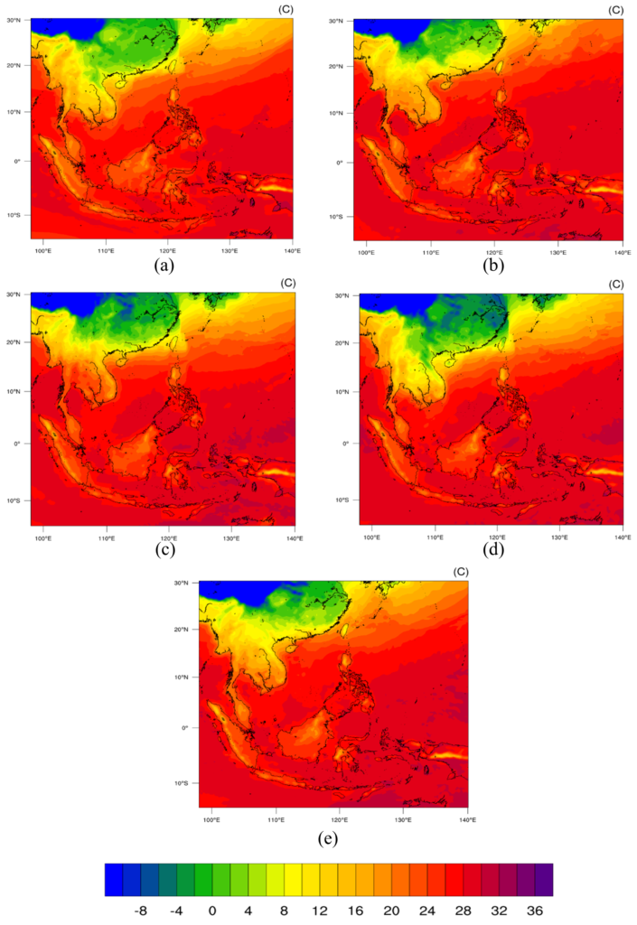
Under RCP4.5, the simulated mean surface temperatures in the SEA region for January of 2013, 2030, 2050, 2070, and 2100 were 22.88°C, 22.51°C, 23.48°C, 23.25°C, and 23.70°C respectively. In July, the mean surface temperatures for the same period were 26.66°C, 26.88°C, 27.43°C, 27.18°C, and 27.59°C, respectively (Table 1). Although the mean surface temperature was simulated to be colder during January 2030 (with a reduction of 0.37°C), the average surface temperature was projected to increase by 0.60–0.82°C during January and by 0.77–0.93°C during July in 2050 and 2100. During January of mid-century, the mainland SEA records a higher temperature change as Cambodia and Thailand set the highest temperature increment with 4.6°C (28.24°C to 32.96°C) and 4.7°C (from 22.08°C to 26.29°C), respectively (Figure 1). Both Myanmar and Laos experienced less significant warming of 0.89°C (from 16.24°C to 17.14°C) and 2.86°C (from 22.83°C to 26.84°C) during the mid-century and became colder at the end of the century with a reduction in the temperature of -5.17°C and -5.14°C, respectively. The mean average surface temperature anomaly toward the end of the century is less pronounced for other SEA countries except for Thailand, which is expected to become colder by 4.49°C.
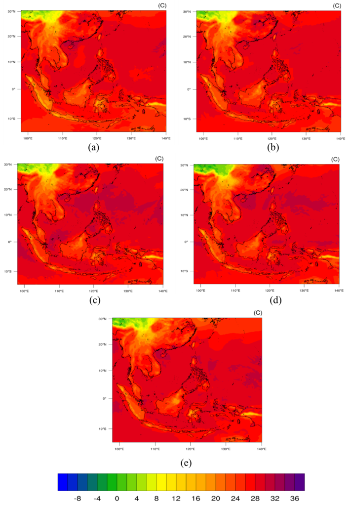
However, during July, the mainland SEA showed a decrement in temperature, while the maritime continent of SEA showed an increment, most notably over the Indonesia region (Figure 2). In 2050, a decrement of 0.28°C (from 30.26°C to 29.98°C) in Vietnam and 0.24°C (from 23.82°C to 23.58°C) in Myanmar were observed. On the other hand, Indonesia showed a significant increment in temperature among SEA countries of 0.83°C (2030), 1.02°C (2050), 1.43°C (2070), and 1.64°C (2100), respectively. Additionally, the result from RCP4.5 also suggests that the surface temperature in mainland SEA is more varied during January compared to July for the entire simulation period. The climate of mainland SEA has a tropical maritime forcing; thus, there is not much surface temperature difference during the dry season (Nguyen, Shimadera, Uranishi, Matsuo, & Kondo, 2019). The tropical forcing (which is a part of global circulation) is an important element that helps to regulate the temperature of mainland SEA by transporting warm air (and replacing them with colder air from the western pacific) into higher latitudes, most notably during the monsoon season (Loo, Billa, & Singh, 2015).
|
Year |
Month |
Surface Temperature (°C) |
Changes (°C) / (%) |
|---|---|---|---|
|
2013 |
January |
22.88 |
– |
|
July |
26.66 |
– |
|
|
2030 |
January |
22.51 |
-0.37 / (-1.62) |
|
July |
26.88 |
0.22 / (0.83) |
|
|
2050 |
January |
23.48 |
0.60 / (2.62) |
|
July |
27.43 |
0.77 / (2.89) |
|
|
2070 |
January |
23.25 |
0.37 / (1.62) |
|
July |
27.18 |
0.52 / (1.95) |
|
|
2100 |
January |
23.70 |
0.82 / (3.58) |
|
July |
27.59 |
0.93 / (3.49) |
The average mean surface temperature under RCP8.5 for January of the years 2013, 2030, 2050, 2070, and 2100 are 23.29°C, 22.95°C, 23.09°C, 24.65°C, and 25.40°C, respectively.
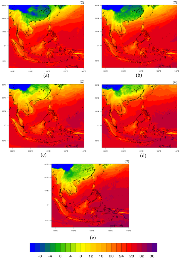
While in July, the mean surface temperature for the respective same year is 26.63°C, 27.39°C, 27.62°C, 28.51°C, and 29.13°C, respectively (Table 2). Like RCP4.5, surface temperature projection under RCP8.5 showed a drop in mean surface temperature in January with a decrement of -0.34°C in 2030 and -0.20°C in 2050. The spatial distribution of surface temperature simulation under RCP8.5 is shown in Figure 3 and Figure 4 for January and July, respectively. The results depict that during January, an increment of surface temperature concentrates over the SEA mainland region during mid-century, with Laos recording the highest temperature increment of 5.74°C (from 21.84°C–27.60°C), followed by Vietnam with 4.29°C (from 22.87°C–27.16°C), Thailand 4.18°C (from 25.46°C–21.28°C) and Cambodia 3.25°C (from 28.27–31.52°C). However, toward the end of the century, the mainland SEA becomes colder while the maritime continent (Indonesia, the Philippines and Malaysia) became warmer with an increment of between 1.63°C and 2.45°C. Seasonal monsoon changes over the region could be responsible for the temperature anomaly during the mid-and end of the century, as discussed by Loo et al. (2015) and (Zhou et al., 2009).
|
Year |
Month |
Surface Temperature (°C) |
Changes (°C) / (%) |
|---|---|---|---|
|
2013 |
January |
23.29 |
– |
|
July |
26.63 |
– |
|
|
2030 |
January |
22.95 |
-0.34 / (-1.45) |
|
July |
27.39 |
0.76 / (2.85) |
|
|
2050 |
January |
23.09 |
-0.20 / (-0.86) |
|
July |
27.62 |
0.99 / (3.72) |
|
|
2070 |
January |
24.65 |
1.36 / (5.83) |
|
July |
28.51 |
1.87 / (7.03) |
|
|
2100 |
January |
25.40 |
2.11 / (9.05) |
|
July |
29.13 |
2.50 / (9.37) |
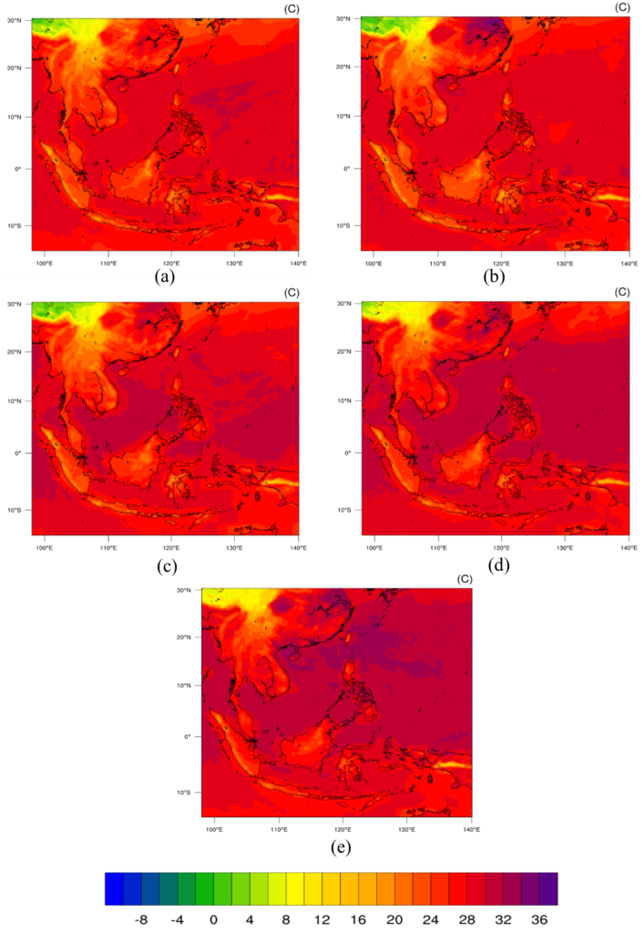
Whereas in July, there was no notable increase in overall mean surface temperature in SEA countries, but the result of the RCP8.5 simulation expected that it would be colder in mid-century with temperature anomalies of -3.50°C in Thailand (from 28.90–25.40), -3.32°C in Laos (from 30.97°C–27.65°C), and -2.15°C over Vietnam (from 31.36°C–29.21°C). Towards the end of the century, the result of RCP8.5 simulations projected that Malaysia, the Philippines, Thailand, and Myanmar would experience warmer changes in temperatures ranging from 1.75°C to 2.28°C. The mainland SEA countries, especially Myanmar, Thailand, Vietnam, Laos and Thailand influenced by the large-scale seasonal reversals of wind regimes (Serreze & Barry, 2011). The two regimes of monsoon are the Southeast Asian summer monsoon (10°–20°N) and the western North Pacific summer monsoon (10°–20°N, 130°–150°E), which are separated by the South China Sea (Kripalani & Kulkarni, 1997). During winter, the tilting of the Earth allows less solar radiation in the northern hemisphere, and this resulted in rapid cooling followed by a pressure decrease in the atmosphere ( Loo et al., 2015). Anti-cyclones develop over Siberia and the cold north-easterly air reaches the coastal waters of China before heading towards Southeast Asia (Malaysian Meteorological Department, 2013).
During the mid-century, there were high-temperature change anomalies projected over the sub-continent region in mainland SEA ranging from 0.88°C to 4.71°C and -3.32°C to 5.74°C under RCP4.5 and RCP8.5, respectively. Meanwhile, the maritime region would experience warmer temperature changes from 0.41°C to 1.16°C and 0.38°C to 0.98°C under RCP4.5 and RCP8.5, respectively. The simulation results also showed a higher temperature increment over the sub-continent region as compared to the earlier finding by Raghavan, Hur, and Liong (2018), which reported increasing between 0.8°C and 1.4°C under both RCP4.5 and RCP8.5 scenarios. However, an earlier study by (Gasparrini et al., 2017) has projected a higher increment of between 3.5°C and 4.5°C at the end of the century for this region. Owing to the uncertainty associated with anticipated temperature changes across climate models and extrapolated climate–response relationships, the estimates of the net surface temperature change over this region might be hampered by poor precision, particularly in places projected to undergo a significant shift in temperature (Almazroui et al., 2020; Dieng et al., 2022) .
3.2 Total precipitation
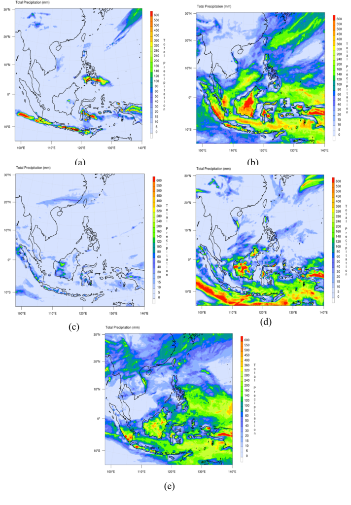
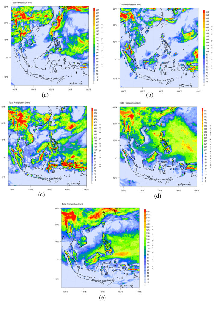
Under RCP4.5, the simulated monthly mean total precipitation in the SEA region for January 2013, 2030, 2050, 2070, and 2100 were 12.57 mm, 80.30 mm, 13.87 mm, 155.63 mm and 135.66 mm, respectively. In July, the mean surface temperatures were 100.53 mm, 90.40 mm, 169.94 mm, 120.23 mm and 90.76 mm, respectively (Table 3). Precipitation analyses under the RCP4.5 scenario showed that the total precipitation of July was higher than January in 2030. The total precipitation projection under RCP4.5 showed changes in the monthly mean of 1.29 mm to 123.08 mm during the January period and between 69.40 mm to -9.76 mm for the July period during the mid-and end-century, respectively. The spatial distributions of projected total precipitation under RCP4.5 are shown in Figures 5 and 6. The results show that total precipitation increments are concentrated over the insular region during January, with pronounced increments after the mid-century. Yet the total precipitation shifted to show an increment over the mainland SEA region during the July period despite having the signal reduced toward the end of the century. As depicted in Figure 5, Indonesia showed the highest total precipitation changes from 41.3 4 mm–284.24 mm, followed by Malaysia with 6.73 mm–225.24 mm and the Philippines from 3.08 mm–184.22 mm during the mid-century and end-of-century periods, respectively. The mainland SEA region only showed a significant increment at the end of the century, with Myanmar setting the highest total precipitation with 242.24 mm, followed by Cambodia (269.45 mm), Laos (160.81 mm) and Vietnam (146.42 mm).
|
Year |
Month |
Total Precipitation (mm) |
Changes (mm) |
|---|---|---|---|
|
2013 |
January |
12.57 |
– |
|
July |
100.53 |
– |
|
|
2030 |
January |
80.30 |
67.72 |
|
July |
90.40 |
-10.12 |
|
|
2050 |
January |
13.87 |
1.29 |
|
July |
169.94 |
69.40 |
|
|
2070 |
January |
155.63 |
143.05 |
|
July |
120.23 |
19.69 |
|
|
2100 |
January |
135.66 |
123.08 |
|
July |
90.76 |
-9.76 |
In July, the total precipitation was simulated to increase over the whole domain area relative to the baseline period. Toward the end of the century, mainland SEA was expected to have a higher amount of precipitation than the insular region during the July period. The entire area receives the most increased total precipitation in 2050, with an increment of 69.40 during the mid-century and a reduction by 9.76 mm at the end of the century. The highest precipitation was observed over Myanmar, with monthly precipitation during July ranging between 131.91 mm–277.39 mm before decreasing to 147.15 mm–177.94 mm at the end of the century. Meanwhile, the rest of the mainland SEA region showed an increment of monthly total precipitation between 62.87 mm–202.92 mm before decreasing by 62.87 mm–105.86 mm at the end of the century (Figure 6). The seasonal total precipitation under the RCP4.5 simulation, particularly during January, was highly varied, especially over Malaysia, Indonesia and the Philippines. The high rainfall over these regions might be caused by the monsoonal winds that transport moisture from the South China Sea and enhance convergence, as discussed in (Tangang, Chung, & Juneng, 2020). Moreover, the high total rainfall, particularly over Malaysia and Indonesia, may also be influenced by the existence of the synoptic Borneo Vortex (Chen, Yen, & Matsumoto, 2013) and the moving oscillation of the Indian Ocean as known as Madden Jullian Oscillation (MJO) (Saragih, Fajarianti, & Winarso, 2018). The MJO and Borneo Vortex phenomena cause this area to become an active area of deep convection associated with heavy rainfall, especially during the wet season.
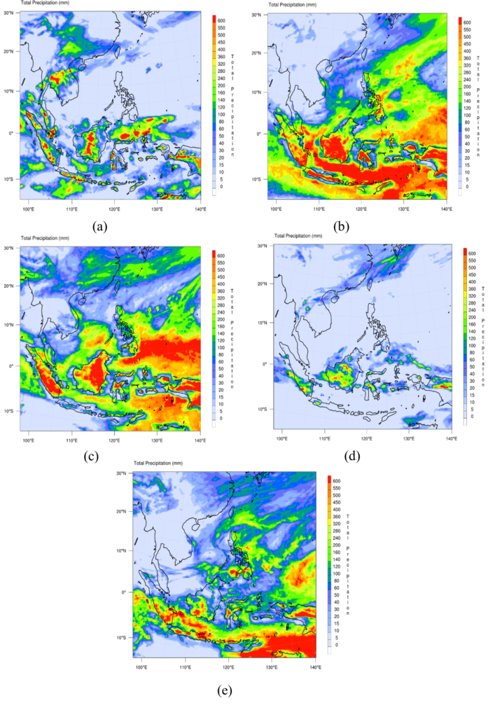
Under the RCP8.5 scenario, the monthly total precipitation in January for SEA was generally lower toward the end of the century compared with the RCP4.5 scenario. The mean total precipitation for January of 2013, 2030, 2050, 2070 and 2100 was projected at 92.98 mm, 169.68 mm, 84.82 mm, 16.10 mm, and 118.79 mm, respectively. While in July, the monthly total precipitation for the respective years was larger than under RCP4.5 simulation but showed a decreasing trend toward the end of the century with total simulated values of 248.86 mm, 258.96 mm, 245.77 mm, 218.25 mm and 92.42 mm, respectively (Table 4). Toward the end of the century, there was no significant increment of total precipitation over mainland SEA during January. However, from spatial distributions of projected total precipitation under RCP8.5 (Figure 7), there was considerable increment over the insular region, particularly toward the mid-century, with the highest increment of total precipitation observed in Indonesia (from 319.33 mm to 332.53 mm) followed by Malaysia (from 215.73 mm to 238.16 mm) and the Philippines (from 135.74 mm to 158.81 mm). A slightly lower marginal increment was observed over the same region toward the end of the century, with total precipitation of 256.67 mm, 51.57 mm, and 193.41 mm for Indonesia, Malaysia and the Philippines.
|
Year |
Month |
Total Precipitation (mm) |
Changes (mm) |
|---|---|---|---|
|
2013 |
January |
92.98 |
– |
|
July |
248.86 |
– |
|
|
2030 |
January |
169.68 |
76.69 |
|
July |
258.96 |
10.09 |
|
|
2050 |
January |
84.82 |
84.82 |
|
July |
245.77 |
-3.09 |
|
|
2070 |
January |
16.10 |
-76.87 |
|
July |
218.25 |
-30.61 |
|
|
2100 |
January |
118.79 |
25.80 |
|
July |
92.42 |
-156.44 |
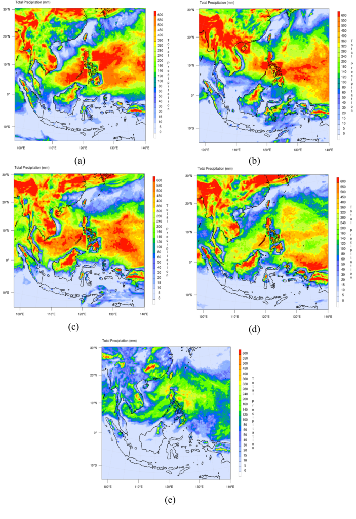
The analyses of total precipitation during the July period (Figure 8) revealed a significant increment of simulated precipitation over mainland SEA despite having the signal reduced toward the end of the century. Myanmar received the highest amount of rainfall with 388.71 mm in 2013, 294.04 mm in mid-century and 85.92 mm at the end of the century. Other regions in mainland SEA showed total precipitation ranging between 209.61 mm–256.06 mm in 2013, 236.46 mm–295.16 mm during mid-century and between 47.38 mm–105.56 mm at the end of the century. Although the insular region follows the same pattern, the simulated total precipitation over the Philippines was an all-time high with 316.57 mm in 2013, 273.27 mm in mid-century and 126.11 mm at the end of the century. In contrast, Indonesia and Malaysia are projected to receive a higher rainfall rate during July by the middle of 91.93 mm and 201.25 mm, but a lower rate at the end of the century, with total rainfall of 9.86 mm and 38.08 mm, respectively. The average surface temperature and total precipitation are recorded as higher anomalies under RCP8.5. These results suggest that significant changes, particularly in the surface temperature and precipitation, could potentially increase this region’s climate-related risks and vulnerability.
The simulated total precipitation in this study was significantly different from the finding of (Tangang et al., 2020) using the CORDEX-SEA multi-model simulation. Their study concluded that the robust significance of total precipitation reduction between 10-30% over maritime sub-continent regions, particularly over the Indonesia region during the dry season (June–August) under RCP4.5 and RCP8.5 by the middle and end of the century. However, during the wet season (December–February), there was a robust increment of 10–20% of the total precipitation observed over Indonesia and a 10–20% reduction over the Philippines in both RCPs. (Tangang et al., 2020) further suggested that the mainland SEA region would experience a 10-15% increment in the total precipitation under both RCPs towards the end of the century except for Vietnam and Cambodia. The higher tendency of drying observed could be associated with enhanced divergence and subsidence effect over the Maritime Continent (Giorgi, Raffaele, & Coppola, 2019) caused by the deep tropical squeeze resulting from the equatorward contraction of the rising branch of the Hadley Circulation as the climate continues to warm (Fu, 2015).
3.3 Climate model evaluation
Table 5 shows the evaluation values of the surface temperature from the WRF model under RCP4.5 and RCP8.5 scenarios relative to the CRU observation dataset. The simulated surface temperature was 25.81°C in January and 27.41°C in July, under RCP4.5. Meanwhile, the RCP8.5 simulation showed a slightly lower temperature of 25.57°C in January and a higher temperature of 27.27°C in July compared with the CRU observation dataset. The model has a lower than 1% bias during January but a higher bias during July with 5.38% and 5.77% for both RCP4.5 and RCP8.5 scenarios, respectively. Meanwhile, the values of FB and NMSE were insignificant. The model has the Fa2 value of 1.0 during the January simulation, indicating an ideal simulation but a slightly higher value during the July simulation with a value of 1.1, indicating a slight overprediction within a factor of two of the observed values. The warm bias over this region could be due to a poor representation of land-atmosphere interactions, amplified by unresolved albedo feedback and further alleviated by large cloud biases (Garrido, González-Rouco, & Vivanco, 2020).
|
Variable
|
Temperature (°C) |
NMB (%)
|
FB
|
NMSE
|
Fa2
|
|
|---|---|---|---|---|---|---|
|
Scenario |
Model |
CRU |
||||
|
|
January |
|||||
|
RCP 4.5 |
25.81 |
25.70 |
0.39 |
0.0038 |
0.00002 |
1.0 |
|
RCP 8.5 |
25.57 |
25.70 |
-0.78 |
-0.0078 |
0.00006 |
1.0 |
|
|
July |
|||||
|
RCP 4.5 |
27.41 |
26.01 |
5.38 |
0.0524 |
0.00275 |
1.1 |
|
RCP 8.5 |
27.27 |
26.01 |
5.77 |
0.0560 |
0.00315 |
1.1 |
Table 6 shows the evaluation values of the total precipitation simulation under both RCPs scenarios relative to the CRU observation dataset. The simulated total precipitations were 29.6 mm and 117.3 mm in January and 159.6 mm and 288.6 mm in July for both RCPs, respectively. There were larger biases for both RCPs, which underestimated the total precipitation during January but overestimated during July. During July, under the RCP4.5 scenario, the values of FB and NMSE were lower than 0.5. Though the model has poor performance in simulating total precipitation during January based on the Fa2 value, it relatively performed well during July with a Fa2 value of 1.3. A similar observation by Kong and Sentian (2015) reported a high bias, especially in the mountainous area and interior region. The larger bias might be caused by poor representation of the convective parameterization and hydrological cycle by the model (Alves & Marengo, 2009; Salimun, Tangang, & Juneng, 2010; Sinha et al., 2013).
|
Variable
|
Precipitation (mm) |
|
NMB ( %) |
FB
|
NMSE
|
Fa2
|
|---|---|---|---|---|---|---|
|
Scenario |
Model |
CRU |
||||
|
|
January |
|||||
|
RCP 4.5 |
29.6 |
244.5 |
-87.89 |
-1.5680 |
6.38120 |
0.1 |
|
RCP 8.5 |
117.3 |
244.5 |
-52.02 |
-0.7031 |
0.56415 |
0.5 |
|
|
July |
|||||
|
RCP 4.5 |
159.6 |
122.4 |
30.39 |
0.2638 |
0.07084 |
1.3 |
|
RCP 8.5 |
288.6 |
122.4 |
135.78 |
0.8087 |
0.78196 |
2.4 |
4. Conclusion
This study concluded that there are connections between climate change and the monsoonal seasonal changes seen in surface temperatures and precipitation, greatly influenced by the weather systems across Southeast Asia. It also shows a significant decadal variation over the precipitation and temperature anomalies. However, the overall temperature in this region showed an increment in the future under both climate change scenarios RCP4.5 and 8.5, which correspond with a decrement of precipitation anomalies for the same period. These shifting phenomena of the monsoon seasons in Southeast Asia will severely impact the region’s vulnerability in human health, environment, food security, and economics. Therefore, policymakers urgently need to mitigate, adapt, and increase climate change resilience in their respective countries.
Acknowledgement
This research was supported by the Asia Pacific Network Research Grant (APN) CRRP2017-02MY-Sentian, in collaboration with Universiti Kebangsaan Malaysia (UKM), University of Philippines Diliman, National Astronomical Research Institute of Thailand, Universitas Palangka Raya, Institute Technology of Bandung, King Mongkut’s Institute of Technology Ladkrabang, National Central University of Taiwan, Malaysia’s Department of Environment (DOE) and Malaysia’s Meteorological Department (METMsia).